Introduction
Generating infinite terrain poses a unique problem in procedural generation since there are no size constraints on what we are generating. With finite generation we can simply create the finite area, generate everything right away, and call it a day. With infinite terrain we obviously cant generate “everything”, so we have to continuously generate a map. To do this we generate finite areas of the map which can be “stitched” together in order to make a practically infinite map. However, one of the biggest challenges with this is having seamless borders between neighboring areas.
Random Generation & Seeding
A fundamental part to generating anything is creating random values. Without random variance we can’t avoid patterns, and while generating patterns is useful in some areas, we wont want it for terrain.
Seeding is what controls the random value generation so that we can replicate random numbers in the exact same order. Seeding is typically done with a single number or string, but can also be done with a set of numbers, which will be useful when seeding an x-y position.
If the seeding function doesn’t allow for multiple seeds, all that needs to be done is to seed using the first number, generate a new random number, add the second seed to the random number, and then seed using the sum. You can repeat this for as many seeds as you need. This does increase how long seeding takes, but its negligible compared to the rest of map generation.
The 3 seeds I use in this project are: The world seed, an x position, and a y position. Seeding is done individually for each region in a map.
Regions
Lets go back to the seamless border problem. Imagine we are generating a segment of our infinite map. We seed for this map, then generate all of the features included in this area. A feature could be a hill, mountain, lake, river, or anything really. Only generating the map using its own features would cause seams between neighboring maps. This is because a feature is big enough to effect neighboring maps, especially if they are close to a border.
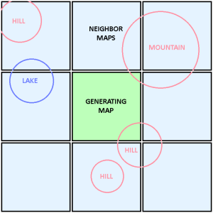
However, this means that for any given map, we would need to process procedures with its 8 neighboring maps, and if the maps are large enough, then many of the procedures we are duplicating wont effect the currently generating map. This is a huge inefficiency since we are increasing our total amount of procedures by 9 times. To fix this, we will divide the map we are generating into regions like so:
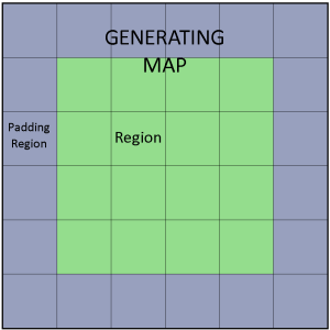
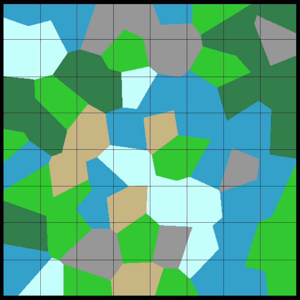
The Green region of our map corresponds to the “usable” area of the map. While the Grey region is padding area which is very likely to effect the usable region. The padding regions is area outside the map, aka the neighboring maps, but now a significantly less amount. Rather than seeding for the whole map, we can seed per region and generate a small amount of terrain features in each region. This means that most of what we generate will be effecting the usable region. In the example picture, there is a 4×4 of inner regions, but that can be increased in order to minimize the proportional area of the padding.
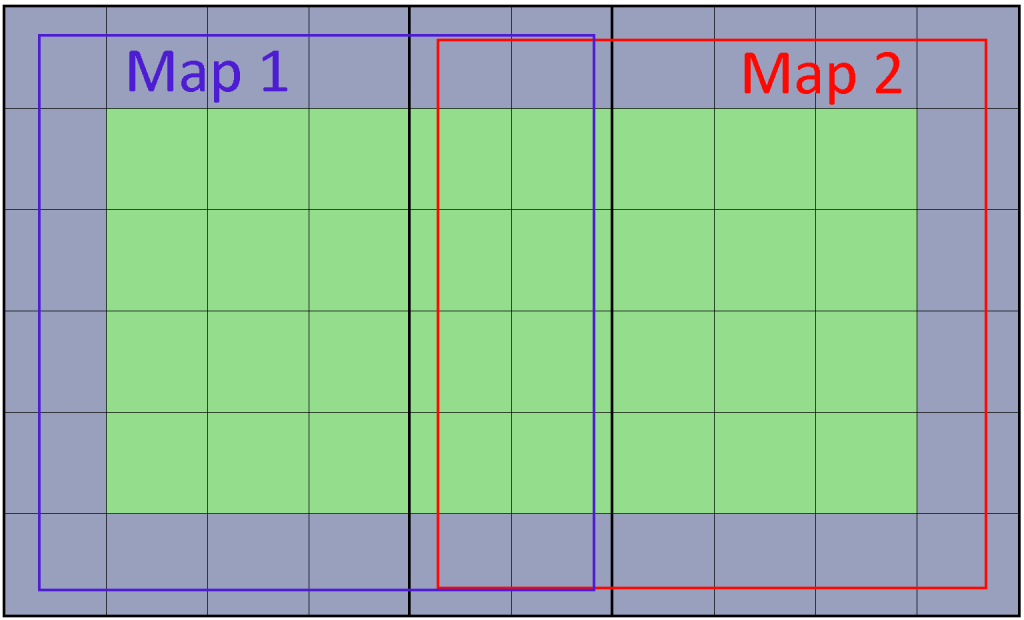
When two maps are combined, the padding area is discarded so that both usable areas are adjacent.
Biomes using Voronoi Noise
Now that the seeding method and setup is out of the way, we can actually start generating things. A simple start is to generate a biome map. A biome map will be a useful start by giving more control for future procedures.
Lets define a region to have the following: a biome type, and a central position. The central position will be a random point in that region’s area. After seeding a region, we use a random number to select the biome type, and another to determine its central position in the region’s area.
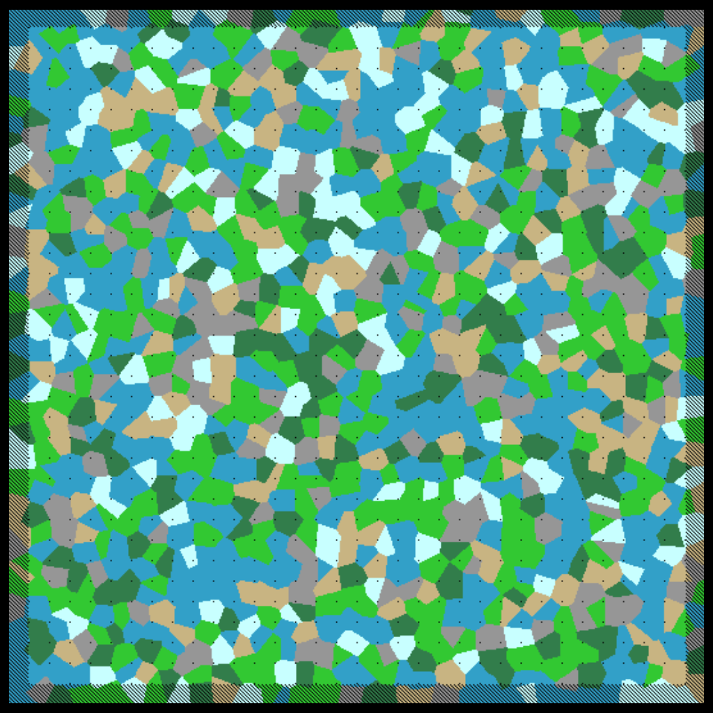
After creating all the regions, we can determine the biome for every position/pixel on the map depending on what region it is closest to. Normally that would just be the biome of the region-grid its inside, but since we defined a central position randomly in the grid it’ll create a voronoi diagram. Creating an image based off of the region of each position on the map would look something like this:
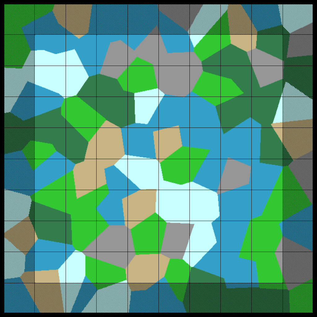
Note that both pictures are the same map with and without padding. To see more clearly the difference between using padding and not, we can generate two neighboring maps and examine their border.

No Padding 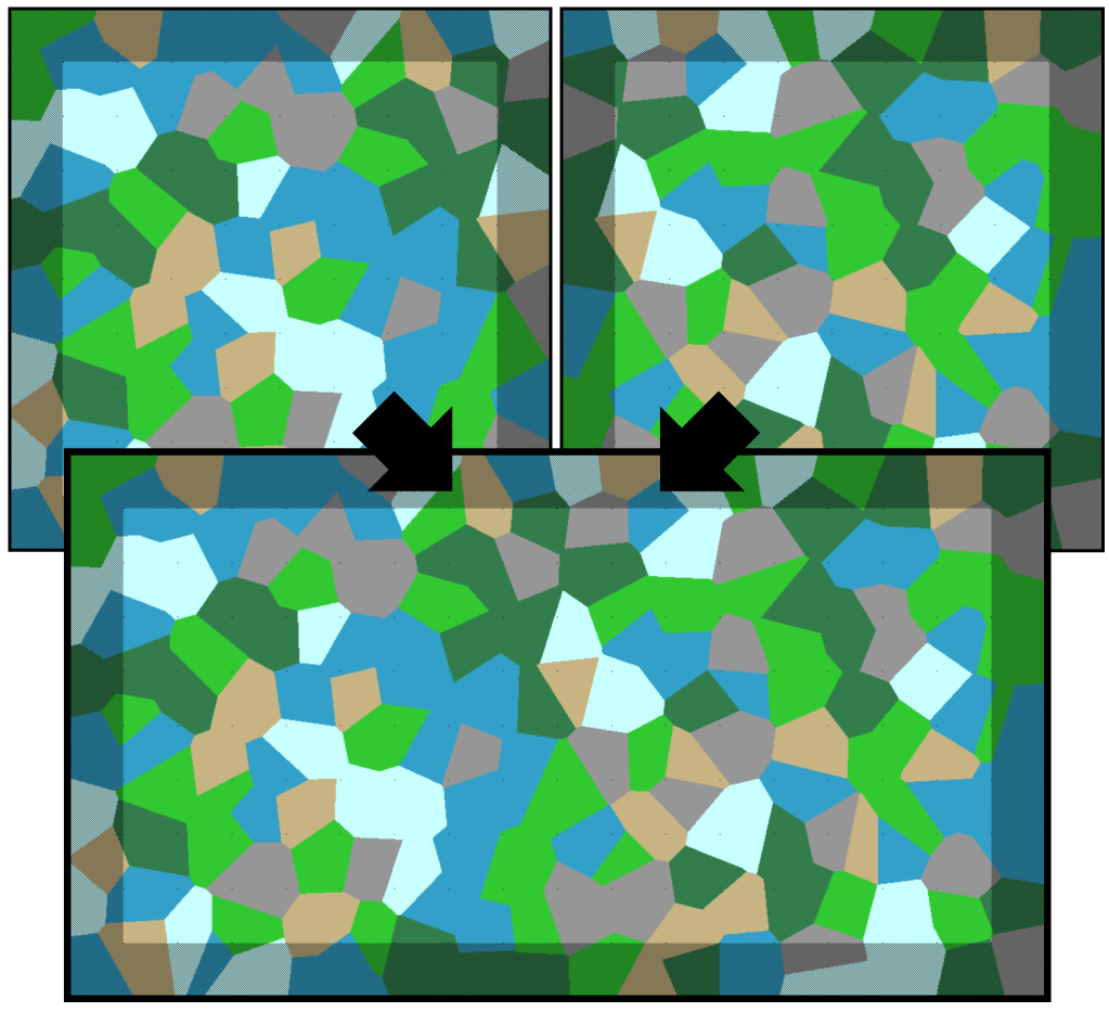
With Padding
As you can see, without padding there is a very noticeable seam along the border between two maps, but the padding regions fix this. Additionally, the reason we only need 1 region of padding around the map is because its impossible for a voronoi cell to to effect a cell two cells away from it, otherwise we would’ve needed a width of 2 regions for padding.
Biome Post-processing
Currently, we only determine the region’s biome based off a random number. It may not appear to be a problem if you don’t have lots of biome types, but it begins to look really messy and rigid really quick. If we generate a map using many regions this becomes extremely apparent.
When creating a region, in addition to getting its biome, we can seed with the adjacent regions to see what biomes surround it. Then you can determine the final biome based on which biome is most occurring, or through other means. Here’s the exact same map, but with this process added on:
Ah, that’s much better! There are plenty of additions to add into region selection. As you can probably tell from above, I don’t have a uniform distribution between all my biomes; there’s a heavy bias to Oceans and Plains. Another addition I added were special cases like the following: If an adjacent region is a “mountain peak” then it guarantees that the biome selected is a mountain. You could even go for a slightly more realistic approach by incorporating temperature to relate neighboring regions together. It’s really fun to mess around with and customize, but you can only go so far with regions alone so its time to use these regions to create a height map!
Height-map Generation
To create the height map I seed for each region, placing “height points” within that region. A height point is simply a 3D point where its x and y position is a random location in the region it’s created in, and a z value which is the height. The height is determined by the biome at that x-y position. The height is another random value determined by a preset range for each biome. The height range also determines if the biome is flat or hilly.
After creating all of the height points, we can generate the height map by taking a weighted average of nearby points for each location on the map. An important part to keep in mind is the region padding again. Since we currently have 1 region of padding, and want a region to only be effected by its close neighbors, we don’t want a height point to effect an area more than 1 region away from it. This can easily be accounted for when taking the weighted average by giving the point an implied radius of 1 region size. If we divide the distance from the height point with the implied radius, we get 0 if the position is directly on the point, 1 if the position is on the outer radius, and more than 1 if further out. We can turn that into a good weight value if we subtract that number from 1 so that there’s a weight of 1 when directly on the point, and 0 on the edge. Although don’t forget to ignore negative weights once past the radius… If we create an image where white is high up, and black is far down, we can see what the height map looks like with a variety of points per region:
1 Point per Region 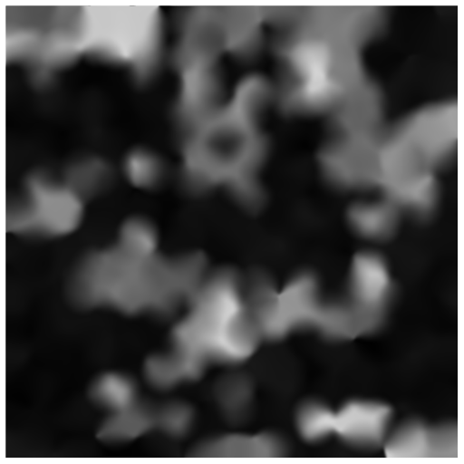
2 Points per Region 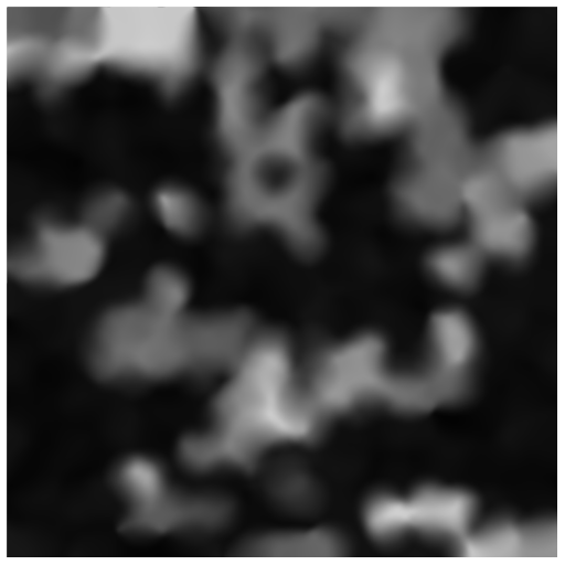
3 Points per Region 
6 Points per Region
As we increase the point count, the weighted average will account for more and more height points which causes it to get blurrier and blurrier. In order to have more points per region while maintaining a good level of sharpness, the implied radius for height points should decrease as more are added. Here’s the same 6 points per region, but with a radius of .75 Region Size:

With this radius tweak, we can see the effects of having 6 points per region; it’s subtle, but the image is sharper than before. We can also overlay this map with our region map to make sure that things are behaving as expected.
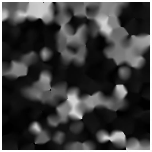
Generating a Normal Map
An additional map that we can generate is a normal map. The only requirement to make one is a height map which we now have. To do this, we go through every location on the height map and use the surrounding 8 locations heights. For each neighbor around the location, we create a 3D axis of two vectors: one vector being the direction from our location to the location of the neighbor, and the second vector being an x-y vector with a z value of 0. For example, if we are looking at our neighbor location that is to the right (x+1), and down one (y-1), our second vector will be [-1, -1, 0] or in general: [y offset, -x offset, 0].
Taking the cross product of this axis and normalizing it will give you a vector that is perpendicular to the slope between the location and neighbor, representing the direction of the surface. Calculate the average normal vector by doing this with all 8 neighbors, and that’s the normal for the location of the map! Finally, we can create an image of the normal map:
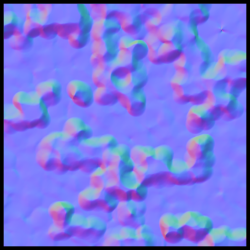
Displaying the normal map also lets us quickly know that the calculations were correct; if different colors are present than its very likely that the second axis vector is wrong or the order of the cross product is flipped.
It’s also a lot easier to analyze the terrain since this is the most 3D representation aside from rendering the map in 3D of course. We can repeat our previous comparisons with the height map, but with the normal map to see things more clearly.
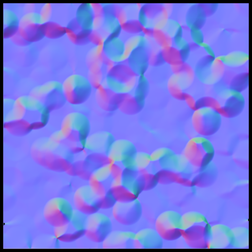
1 Point 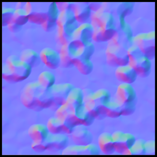
3 Point 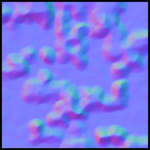
6 Point 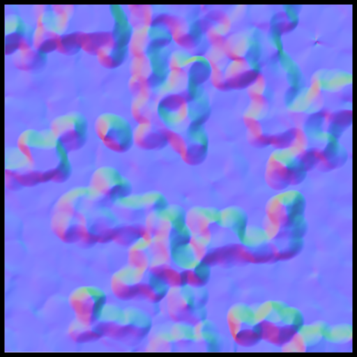
6 Point with .75 Radius
Now we can clearly see the differences between the 6 Point, and the 6 Point with a smaller height point radius. We can also see more benefits to having more points such as how the circular shapes caused by the way we calculate heights is less prevalent.
Generating a Preview Image
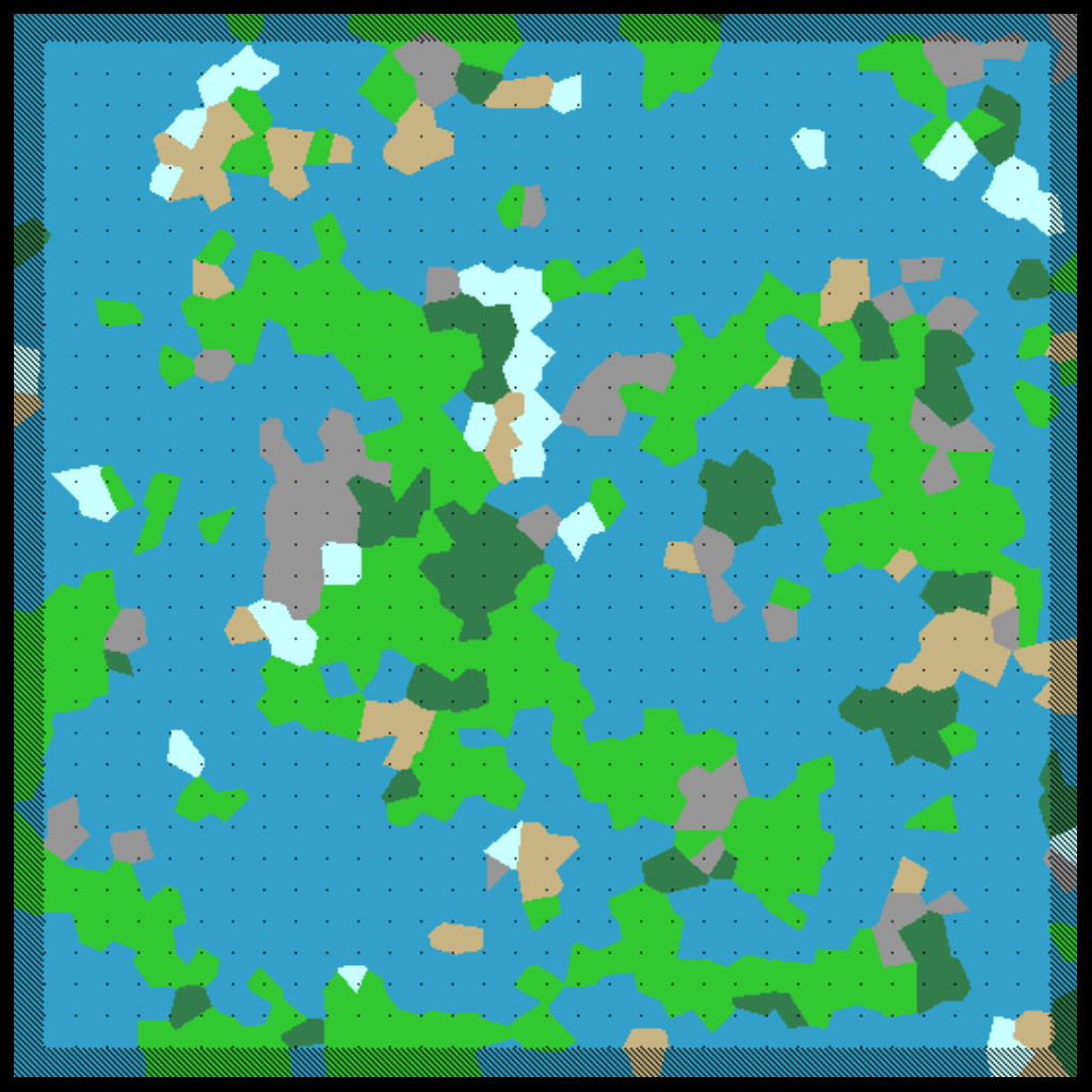
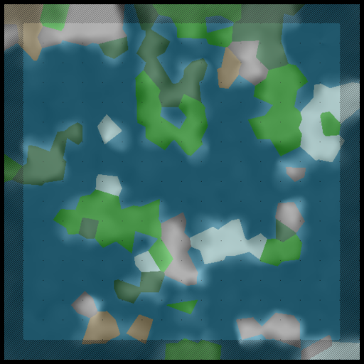
Using all of our maps as input, we can generate a simple preview image to get an idea of what the world might look like. The color selection will be similar to the region map, but we can add certain conditions based on the elevation. So we can define a water level where heights under the elevation will be blue, and for certain regions, put sand at the shoreline near water level. For mountain regions, I color it white if it gets high enough. We can also use the normal map to find steep cliffs and color them grey to show cliff sides clearer too. To do this we do a dot product with the normal vector and the up-vector. If the dot product is 1, the surface is upright, if it is 0, its a straight cliff. If the dot product is less than .5, I color it a cliff. Finally we can darken the color based on the height. With all of that we can get an image that looks like this:
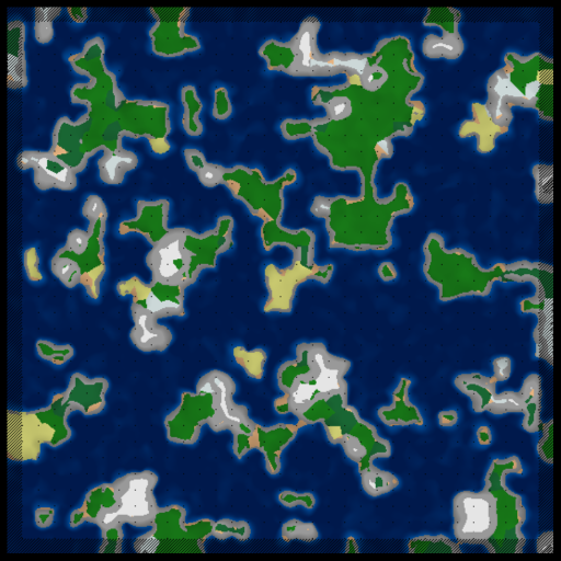
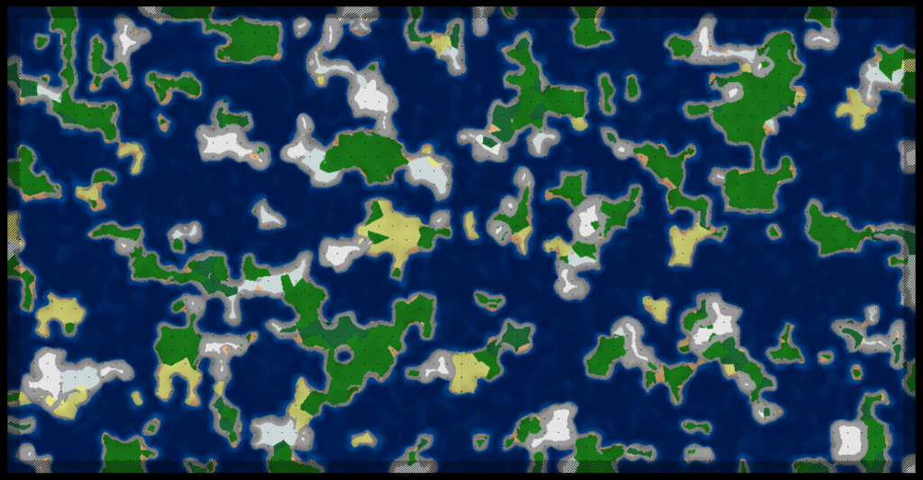
And just to be sure, we can make sure that they are seamless by joining adjacent maps:
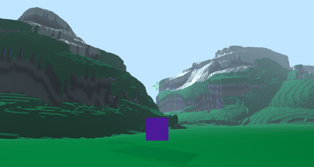
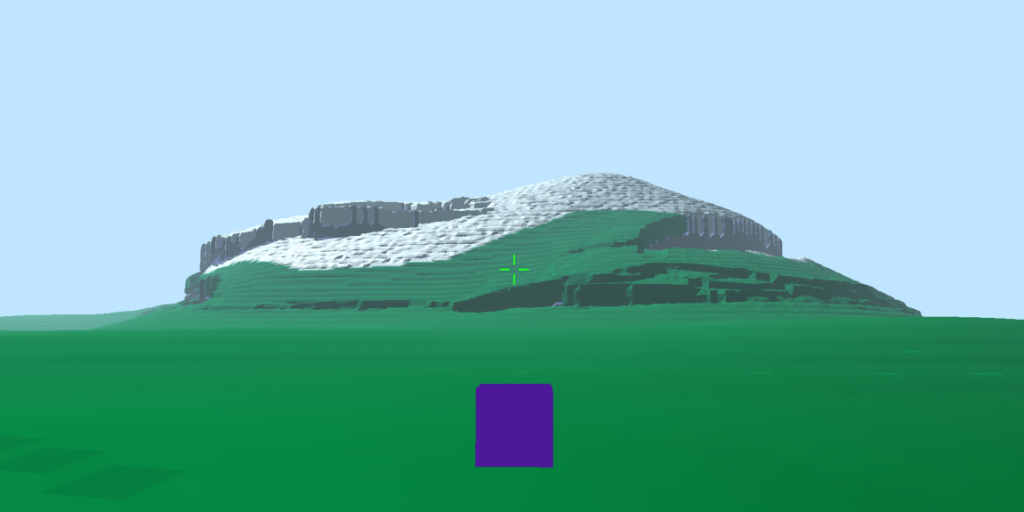
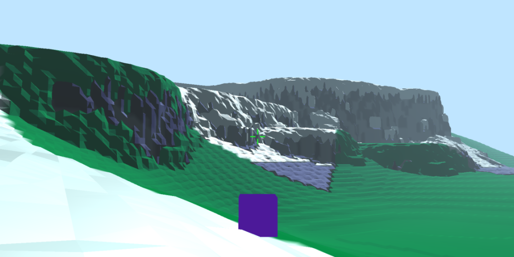
Generating in a 3D environment
After adding a few more procedures like terracing, I generated a mesh using the heightmaps and marching cubes. Here are some screenshots:

Conclusion
Since my goal was to handle infinite terrain generation, this approach satisfied that. However, this specific approach has pros and cons to it. If you’ve seen other terrain tutorials you’ve definitely heard of Perlin noise. Perlin noise can also be used to solve the issue of seamlessness because is can already give you any arbitrary value for an x-y position such that its neighbors are similar values. This means you wouldn’t need to set up and deal with seeding regions for efficient procedure processing. However, using Perlin noise as a foundation means that every following procedure also needs to behave similarly which can end up as a big restriction. If you want fast results, both in development time and runtime generation, Perlin noise is a good pick. However, if you want to trade that out for more control over you procedures this seeding method isn’t a bad pick.
This project was mainly a proof of concept as well as a challenge to see what I could come up with on my own, but I did reuse this seeding method for another project which utilizes the control a bit more by aiming to create a world with a touch of level design.
